No macros are required. There is a setting item in the PowerQuery editor, but the setting is difficult to find.
If the CSV data from the core system contains carriage returns, the columns will shift. It would be nice if we could controle the system easiliy, but sometimes we could not. That’s the solution.
If you use this method, CSV with line breaks in cells can be opened in Excel without collapsing the table.
It is also recommended for non-programmers because it can be operated from the menu without writing complicated code.
Importing from “From text/CSV” and Importing from a “folder” will have different settings, so I will explain each.
In case inporting “From text / CSV”
Operating procedure
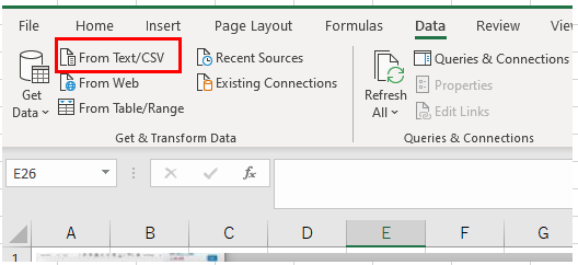
Click “Data”-> “From text / CSV” on the menu bar.
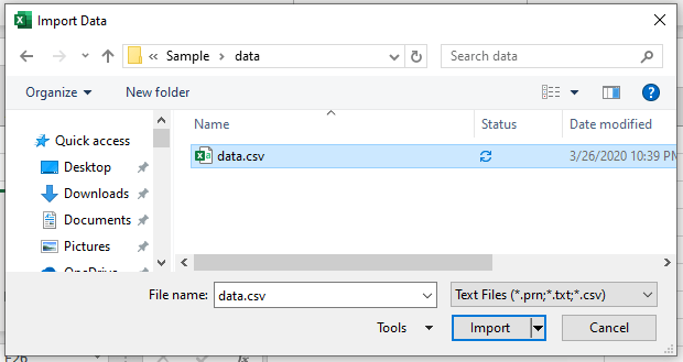
Select the CSV to read and click “Import“. (Select CSV to open but change to import)
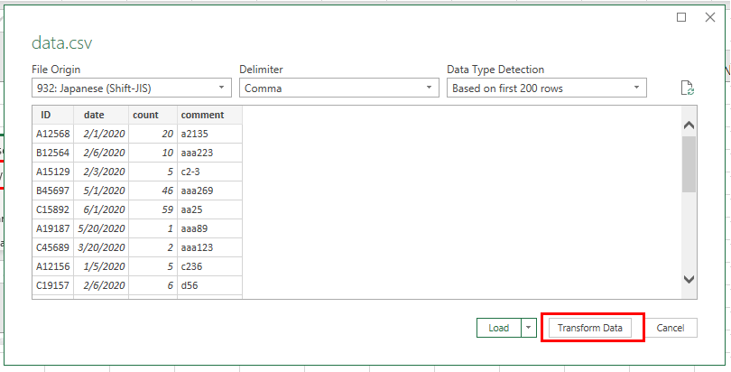
Click “Transform Data“.
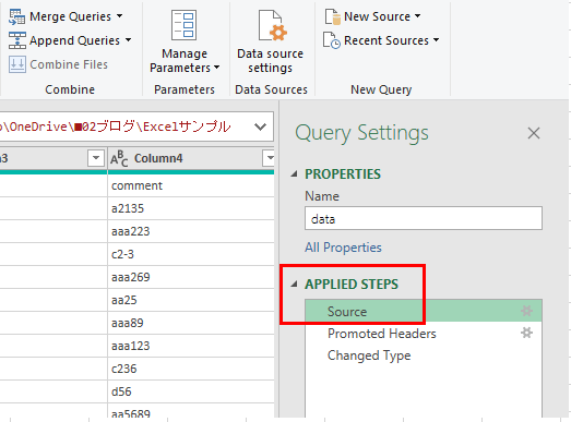
When the power query editor starts, double-click “Source” in “Applied steps“.
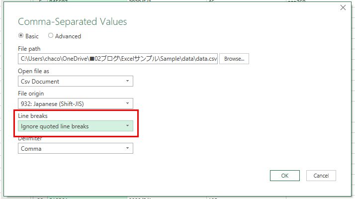
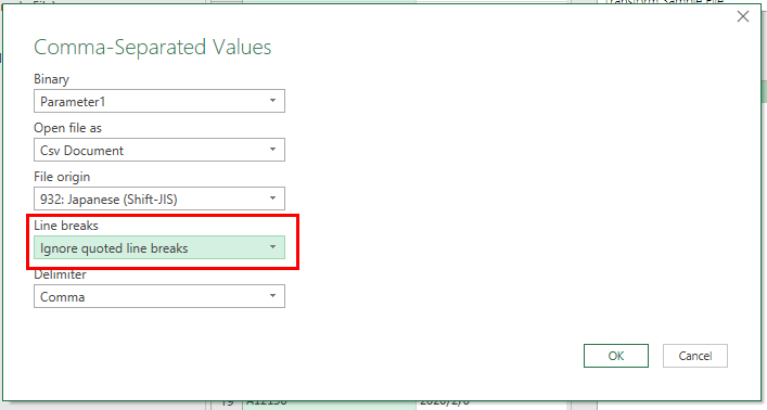
When the “Comma Separated Values” window opens, select “Ignore quoted line breaks” from the pull-down under “Line breaks” and click “OK”.
When you return to the PowerQuery Editor, click “Close and Load” in the upper left.
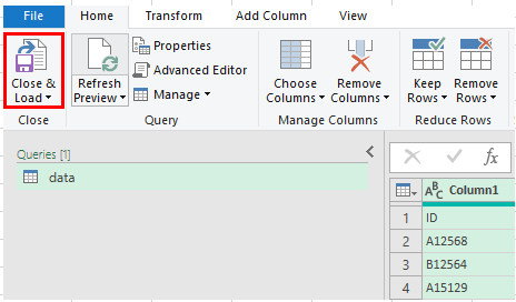
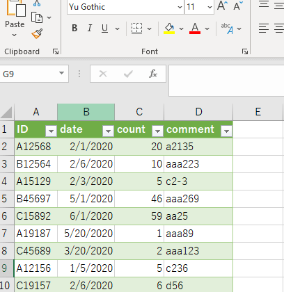
The CSV has been loaded into the worksheet.
That is all for reading from text or CSV.
In case importing “From folder”
Operating procedure
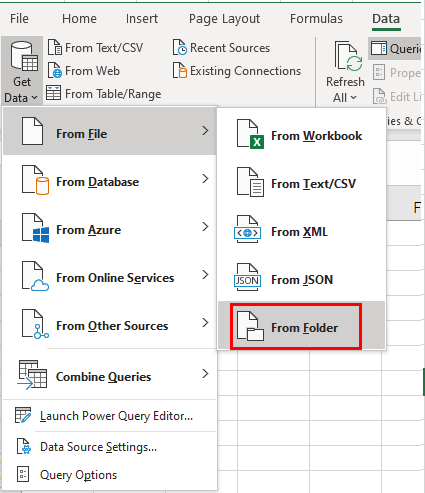
Click “Data“->”Get Data” ->”From File“-> “From Folder” on the menu bar.
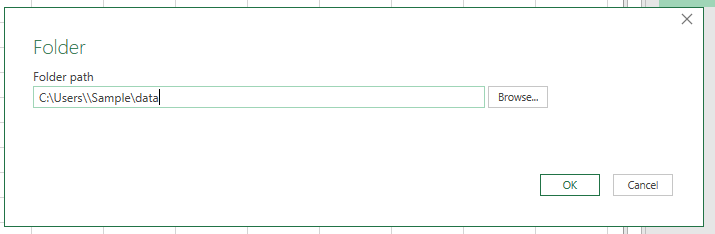
Click “Browse”, select a folder to save the CSV, and click “OK”.
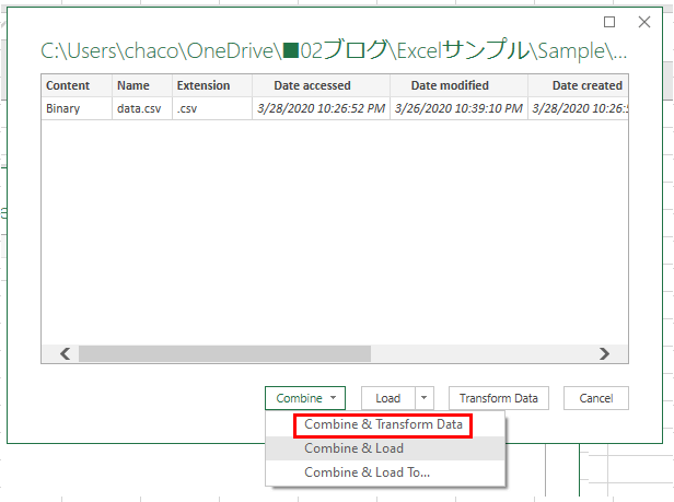
Click “Combine” ->”Combine & Transform Data“.
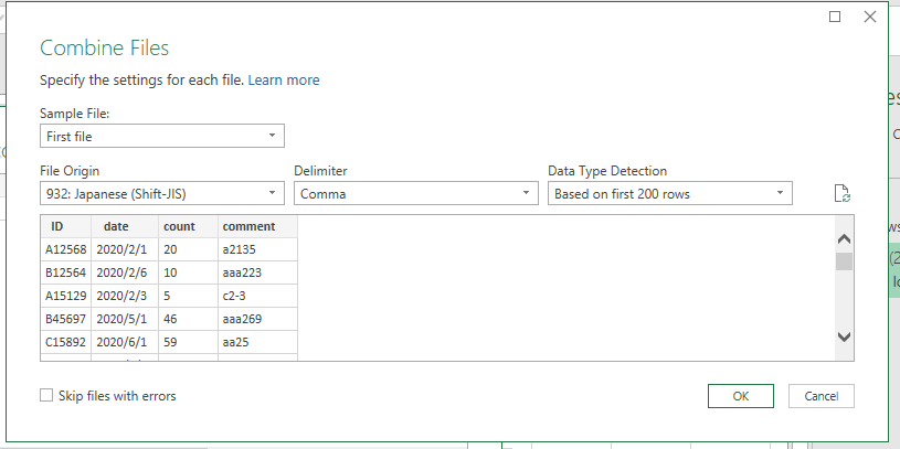
 Click OK for Combine File.
Click “Transform Sample file” and double-click “Source” from “Applied Steps” on the right.
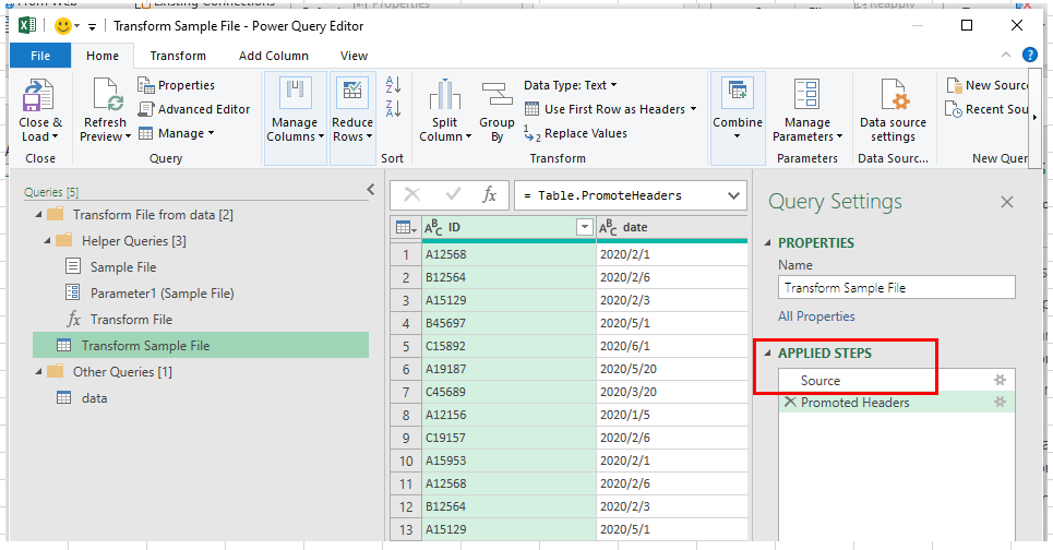
[aside type=”normal”]In this case, the query loaded into the worksheet is a query named “Data”, but the setting is “Conversion of sample file” in the middle. Here is the difference from the previous method. [/aside]
When the “Comma-Separated Values” window opens, select “Ignore quoted line breaks” from the pull-down under “Line breaks” and click “OK”.
When you return to the PowerQuery Editor, click “Close and Load” in the upper left.
The CSV has been loaded into the worksheet.
That’s all for reading from a folder.
To open the PowerQuery editor after import
If the worksheet is already expanded after importing, open the PowerQuery editor as follows:
Click “Data”-> “Get Data”-> “Launch PowerQuery Editor” on the menu bar. Then double-click on the step item as described above.
Once you make it, you can update it all with one button
The “from folder” function of “Get & Transform Data” is incredibly useful. Regardless of whether the file name changes or the number of files changes, the files are combined (UNION combination) and imported without concern.
It is very convenient because once you have set it, you can perform everything from importing data to tallying with one button of “Update All”. I also make full use of it.
“Get & Transform Data” are like blueprint. The procedure seems cumbersome, but once you make it, replace the original data and update it all with the “Update All” button. Furthermore, if you make a pivot table based on this table, you can even make a summary table.
For example, by downloading data that changes every day of the system every morning and saving it in a predetermined folder, the sales amount, number of items, progress, etc. can be updated with one button. I have started and updated about 10 files in a row with VBA, and I am empty-handed for about 1 hour every morning. Accurate over explosive speed. In the meantime, you can check emails, contact business, and replenish hot water in the pot.
Like this
- Replace the CSV of the original data (Delete the old file and save the new file. OK even if the file name and name change. However, the number of columns and title should be the same format)
- Open the Excel file for which “Get & Transform Data” have been set.
- Click Data → Update All. The worksheet table is updated.
* In addition, I download and upload are automated in the every morning.
Afterword
Until I found this method, I used to open the file once in Excel, remove the line feed code with a macro, and save it as CSV.
The benefits of “Get & Transform Data” are many. For example, data can be extracted by specifying conditions even from CSV that exceeds the number of rows that Excel can handle. In fact, the data I am dealing with is well over 1.04 million.
“Get & Transform Data” was terrific, and we analyzed over 430 columns of data last year, over 2 million rows, but I did. It is over 4GB in csv. I’m not boasting a few things, but just for your reference.
However, naturally, please note that the data after extraction cannot exceed the number of rows handled (Excel cannot Load it).
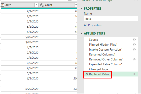
By the way, special characters such as line feed codes can be replaced with PowerQuery.
How to replace
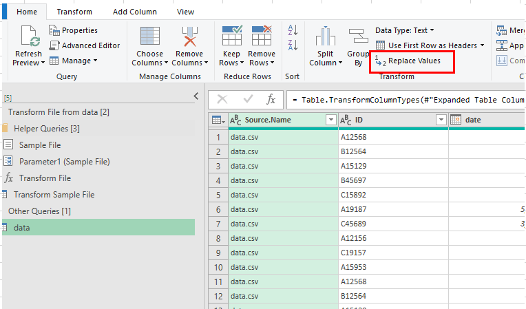
Select the column which you will convert on Power Query Editor. the Click “Replace Values” from “Home” in the menu bar.
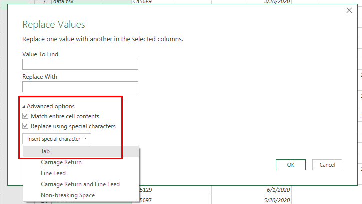
Click Advanced Options.
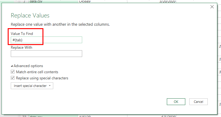
In the window that opens, check “Match entire cell contents” (required). Check “Replace with special characters” and click “Insert special characters”. Click “Tab” from the pull-down menu.
Japanese version